Total Return or Bust Part II: Using Bond Yields to Estimate Total Returns with Pandas and Numpy Financial

Finance Topics Covered

Estimating fixed income total return using historical yield data.

Technical Skills Used

pandas, pandas datareader

numpy, numpy financial

matplotlib

Welcome to Total Returns Part II! The rare sequel that’s better than the original, entering the rarified air of Empire Strikes Back, Terminator II, Back to the Future II, and Top Gun: Maverick (triggered?).

In the last post, we got a sense for why focusing on total return is important, and how to apply that to equities. Today, we are going to learn how to estimate the total return on fixed income securities. Yay! Bonds!

Often we’ll see arm chair pundits on fintwit post yield charts and talk about how bond investors are suffering, and that doesn’t always map to the lived experience of actually holding those bonds. Similarly,

Another huge motivation for using yields to estimate total returns is that it unlocks decades of additional data for us. There really isn’t a lot of reliable and accessible data on bond prices and returns extending back before the 90’s, especially if you’re a retail investor. (At my last gig, JP Morgan quoted us $15k for an annual subscription to their emerging market bond index data 🙃.)

This entire period was also one of generally declining rates, opening us up to huge out-of-sample risk if we only have a narrow band of economic regimes to analyze. However, we do have data on yields that extends back deep into the 20th century. The FRED data we’ll tap into today goes back to 1962, but there are other sources like Robert Schiller’s data at Yale where you can find yields back into the 1910’s. This vastly expands the variety of economic and interest rate regimes we can analyze in terms of their impact on financial assets. We can now estimate the actual impact the inflationary periods in the 1970’s had on financial assets, for example.

Quick caveat: these are estimated returns based on the assumption that we are pricing and buying a brand new bond of a given maturity at the beginning of each month and holding it for one month before selling and buying another brand new bond priced at par using the prevailing market yield. This is stylized and does not directly represent reality — the Treasury does not issue new ten year bonds every month! Nor does this include transaction costs. Simplifying assumptions aside, this is still a useful tool to have in the toolkit for conducting long term historical analysis of financial markets.

Let’s get into the code.

Pretty standard import list. If you don’t have pandas datareader or numpy financial installed in your working environment, you can do so easily via pip. For convenience, you can head to the mortgage affordability post and copy those commands directly. 🤙🏼


import pandas as pd
import numpy as np
import pandas_datareader as pdr
import numpy_financial as npf

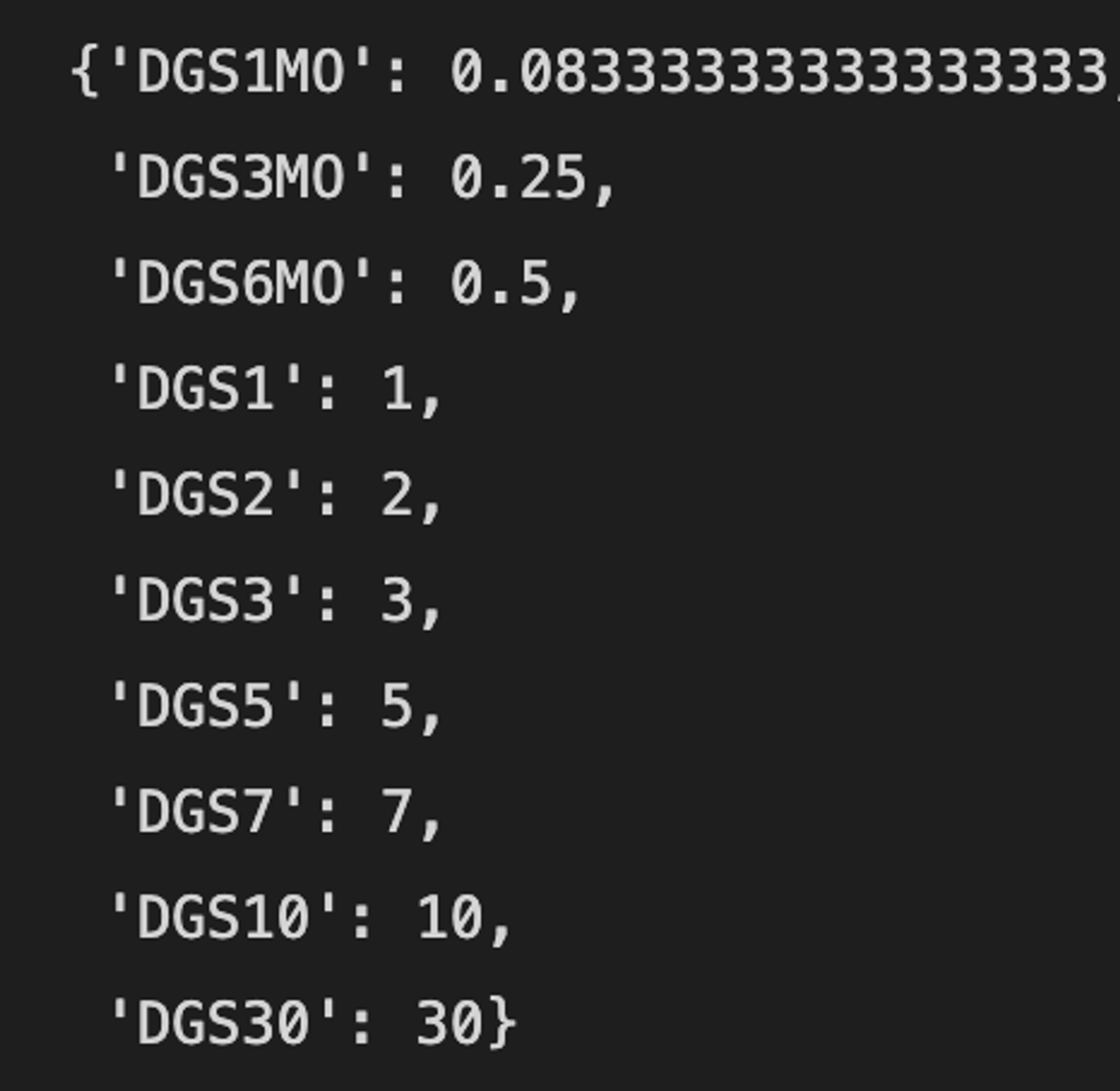
Next, we’ll initialize some lists with the FRED time series identifier for each Treasury bill/note/bond and their corresponding tenor expressed as a number.


maturities = [
    "DGS1MO",
    "DGS3MO",
    "DGS6MO",
    "DGS1",
    "DGS2",
    "DGS3",
    "DGS5",
    "DGS7",
    "DGS10",
    "DGS30",
]

tenors = [1 / 12, 0.25, 0.5, 1, 2, 3, 5, 7, 10, 30]

symbol_tenor_map = dict(zip(maturities, tenors))

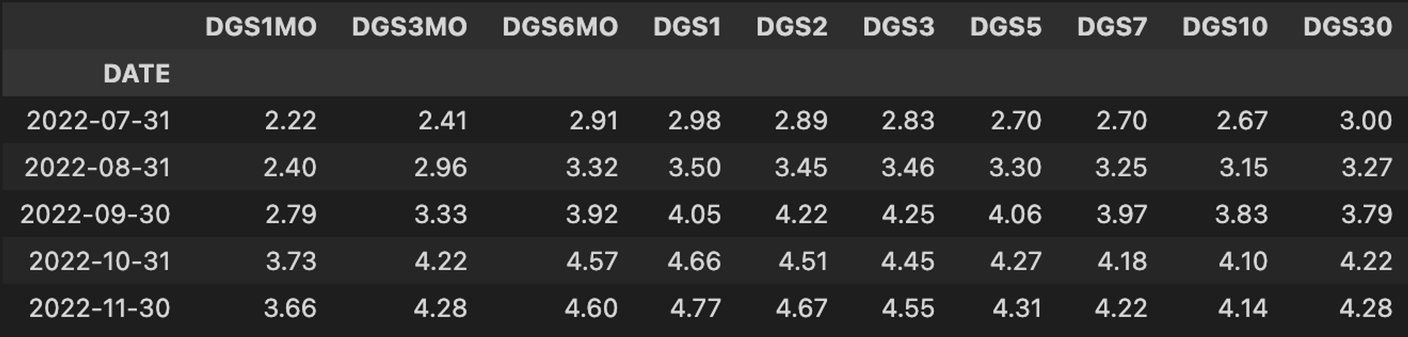
Let’s kick things off by pulling in our initial dataset with an api call to FRED. We are going to be estimating monthly returns, so we’ll chain the resample method to grab the last value for each month.


yields = pdr.DataReader(maturities, "fred", "1900-01-01").resample('M').last()
yields.tail()

Source: FRED. Also, can you spot the inverted yield curve?

Now that we have our yields let’s take a little aside and review some bond basics.

Bond prices have two components: the present value of future coupon and principal payments, and the accrued interest from the previous coupon date to the date of pricing. Thus, you’ll often see two types of prices quoted for bonds:

Flat Price: the present value component

Dirty Price: Present Value + Accrued Interest

For the first part of this tutorial, we are going to break out the calculation into its component parts using the 10-year Treasury Note as an example. Then, we’ll generalize it into a handy function that accepts the yield series and tenor as arguments and spits out the total return. We can then use that function to generate a total return history for the entire yield curve. How neat is that?

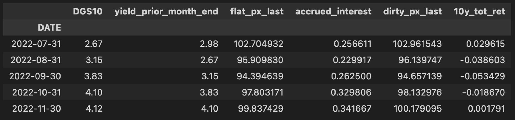
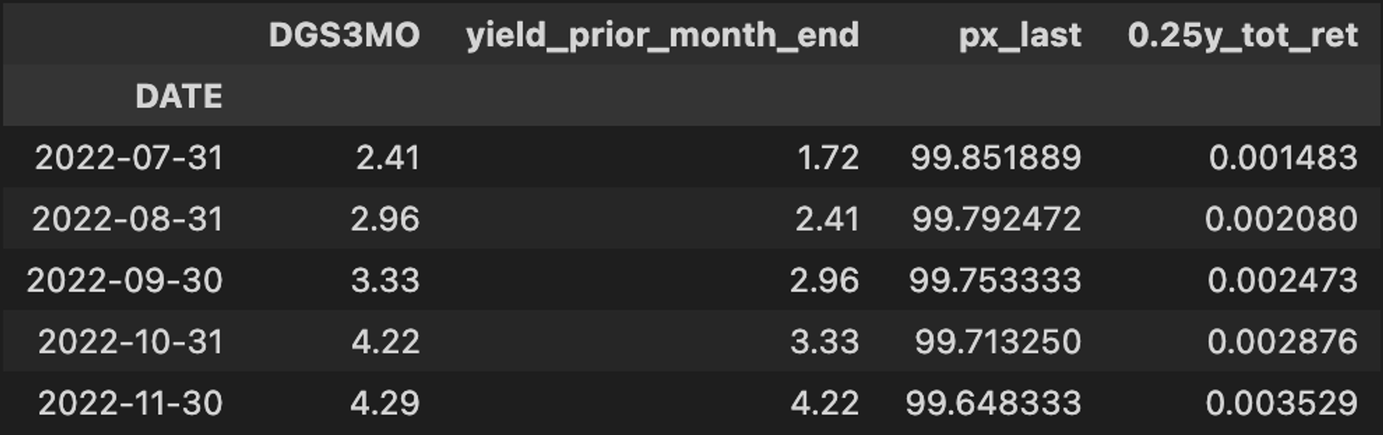
First, we’ll grab our ten year yields, convert it from a Series to a DataFrame, and add another column with the previous month end’s yield.


tens = yields['DGS10'].to_frame()
tens.loc[:,'yield_prior_month_end'] = tens.shift(1)

Next, to be precise in our accrued calculations we are going to create an array that measures the length of each month, expressed in days. Probably fine to just plug 30 for this, but it’s fun to be extra and also is the perfect application for working with the np.timedelta64 function.


interval = (tens.index - tens.index.shift(-1)) / np.timedelta64(1, "D")

Our next block should look mostly familiar to anyone who’s ever calculated the present value of something before (TI BA-II maxi here).

Coupon payments are made semi-annually. So, for a bond maturing in ten years, our nper is 20 and our iy is half of the yield value (expressed as a decimal).

Our pmt for a month is half of the prior month’s yield, and the accrued interest earned in a month is the length of that month divided by the accrual period of 180 days, multiplied by the coupon payment.


nper = symbol_tenor_map['DGS10'] * 2
iy = tens.iloc[:, 0] / 100 / 2
pmt = tens["yield_prior_month_end"] / 2
ai = interval / 180 * pmt

Unlike my humble BA-II Plus, we aren’t limited to calculating one present value at a time, we can take advantage of vectorized operations in numpy and pandas. Here, we are taking our outputs from the previous block, and passing them into the npf.pv function to price a ten year bond at par using the prevailing market yield each month. Adding the accrued interest gives us our full aka dirty bond price for each month.


tens.loc[:, "flat_px_last"] = (npf.pv(iy, nper, pmt, 100)) * -1
tens.loc[:, "dirty_px_last"] = yields["flat_px_last"] + ai

Almost therrre! Last step is to calculate a simple month-over-month percentage change. We can use f-strings in conjunction with the symbol_tenor_map we defined earlier to dynamically name our final total return column.


tens.loc[:, f"{symbol_tenor_map['DGS10']}y_tot_ret"] = yields["dirty_px_last"] / 100 - 1

Let’s take a look at the full result. Recall, we are modeling a hypothetical scenario where we buy a ten-year bond prices at par (100.00) at the beginning of the month at the prevailing market yield, and then sell that bond at the end of the month at the new yield, repeating that process each month.

Tenors less than one year don’t pay coupon payments. Instead the bill is discounted at the prevailing yield and then redeemed at par upon maturity, so we’ll need to handle these differently.

💡

Bill yields (and fixed income securities more broadly) are always quoted on an annual basis. For example, if the 3-Month Treasury Bill yields 4% (still can’t believe that’s become a reasonable example), that implies that you would earn 4% if you bought and held four 3-Month bills over the course of the year.

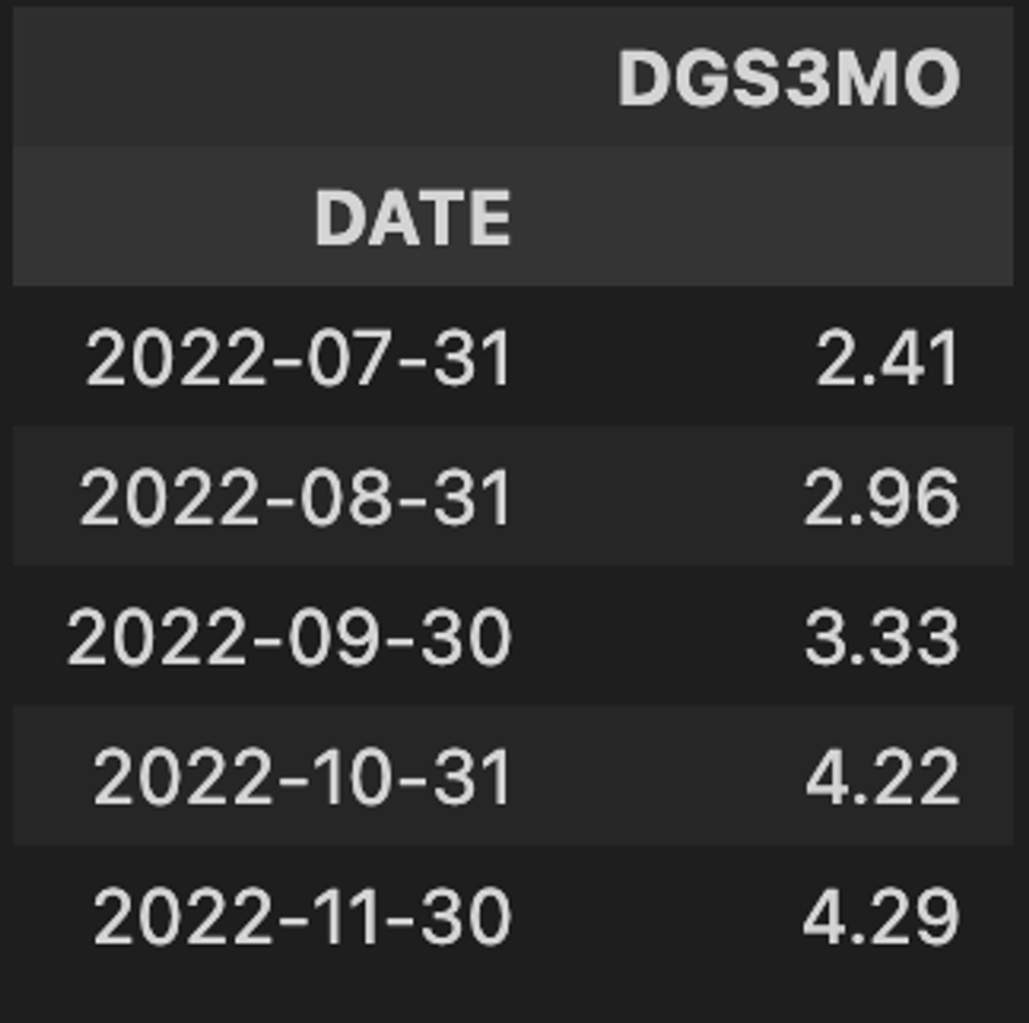
Let’s grab the historical yields for the 3-Month Treasury bill to demonstrate this piece.


bills_3m = yields['DGS3MO'].to_frame()
bills_3m.loc[:, "yield_prior_month_end"] = bills_3m.shift(1)
bills_3m.tail()

This simplifies our approach — we just need to use our interval variable to get the precise fraction of a year (360 days is often used in fixed income land to represent a year), then multiply that by our annual yield from the prior month and subtract from 100 to get the discounted dollar price. The return over the previous month is then 100 divided by last months discounted price.


bills_3m.loc[:, "px_last"] = (
		100 - bills_3m["yield_prior_month_end"] * (interval / 360)
)


bills_3m.loc[:, f"{symbol_tenor_map['DGS3MO']}y_tot_ret"] = (
		100 / bills_3m["px_last"] - 1
)

Let’s generalize this into a function. We can add some conditional logic based on the tenor to determine which of the two calculation methods we need to perform.


def bondTR(yields, tenor):
		"""
			 takes a pandas Series of yields and the tenor expressed numerically 
			 and returns a DataFrame with price and total return calaculations in
			 in addition to the original data.
		"""  
    yields = yields.to_frame()
    yields.loc[:, "yield_prior_month_end"] = yields.shift(1)
    interval = (tens.index - tens.index.shift(-1)) / np.timedelta64(1, "D")
    if tenor > 1:
        nper = tenor * 2
        iy = yields.iloc[:, 0] / 100 / 2
        pmt = yields["yield_prior_month_end"] / 2
        ai = interval / 180 * pmt
        yields.loc[:, "flat_px_last"] = (npf.pv(iy, nper, pmt, 100)) * -1
        yields.loc[:, "dirty_px_last"] = yields["flat_px_last"] + ai
        yields.loc[:, f"{tenor}y_tot_ret"] = yields["dirty_px_last"] / 100 - 1
    else:
        yields.loc[:, "px_last"] = 100 - yields["yield_prior_month_end"] * (interval / 360)
        yields.loc[:, f"{tenor}y_tot_ret"] = 100 / yields["px_last"] - 1
    return yields[f"{tenor}y_tot_ret"].dropna()

You’ll notice we’re just returning the final total return column in this function. We wouldn’t need to store all of the intermediate steps if peak efficiency was the goal, but they’re left in here to illustrate how our individual steps come together. In human time, it’s still lightning fast. The function could easily be modified to return either a) the whole DataFrame for a given yield, or b) not retain any of the intermediate columns and return only the final total return calculation.

We can use our function to total returns for one tenor of interest…


tens_tr = bondTR(yields['DGS10'], symbol_tenor_map['DGS10'])

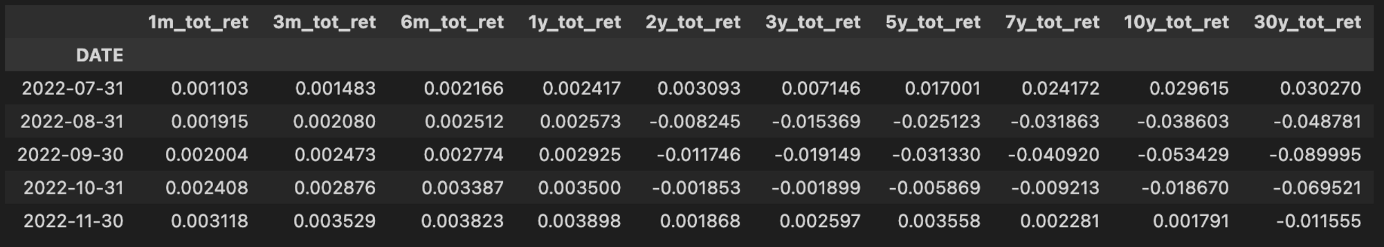
… or wrap it with pd.concat and some list comprehension to generate a DataFrame with total return estimates across all tenors.


trs = pd.concat(
    [
        bondTR(yields[key], symbol_tenor_map[key])
        for key in symbol_tenor_map.keys()
    ],
    axis=1
).rename( # tidy up the bill column labels
    columns=
        {
            f"{1/12}y_tot_ret":"1m_tot_ret",
            f"0.25y_tot_ret":"3m_tot_ret",
					  f"0.5y_tot_ret":"6m_tot_ret"
        }
)
trs.tail()

Source: Author’s calculations, FRED data.

Be Extra — Yield Curve Inversions, Recessions, and Total Returns

Let’s be extra and put the latest bond rout into historical perspective. We’re going to look at the total return of the ten-year note over time, as well as the slope of the yield curve measured by taking the ten-year yield and subtracting the two-year yield.

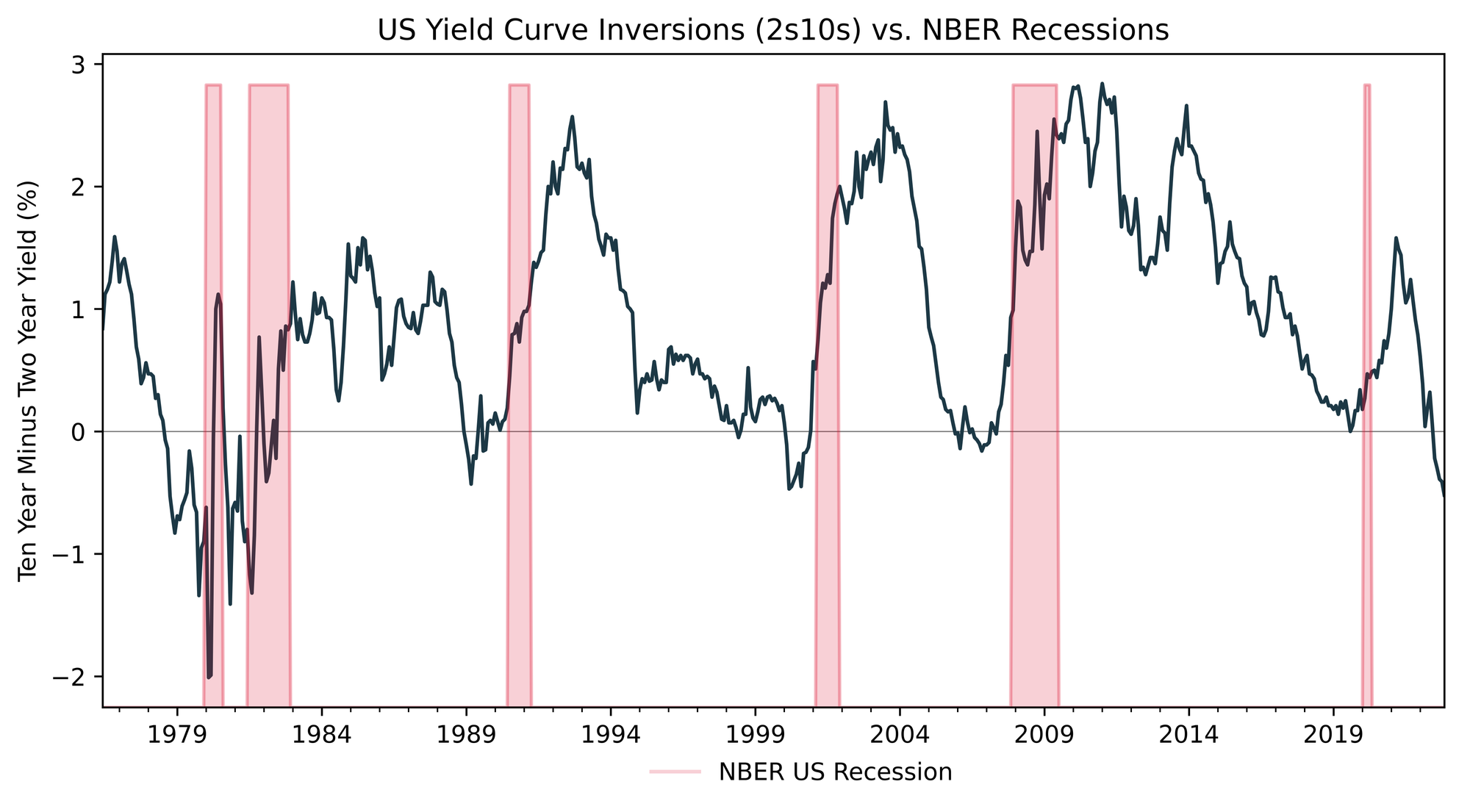
Yield curve inversions have an established track record of portending recessions, albeit with a long and variable lag. Many explanations have been offered up as to why curve inversions generally lead recessions. One that I tend to subscribe to is that an inverted curve threatens the profitability of core banking activities in the economy. Banks make money by borrowing short term (eg. demand deposits, commercial paper) and lending long term (eg. mortgages, industrial loans). When the curve is not inverted, all is good in the hood, as the banks enjoy a positive net interest margin. When the curve inverts, this activity becomes unprofitable, and banks shift their focus to tightening credit standards and reducing lending. Obviously in the complex adaptive system that is the global economy, there is an iceberg of nuance and other variables below this, but I think this is an intuitive and useful mental model.

We’ll start the second part of our quest by gathering the necessary data.


twos_tens = (yields['DGS10'] - yields['DGS2']).dropna()
tens_tr = bondTR(yields['DGS10'], symbol_tenor_map['DGS10'])
tens_tr_12m = tens_tr.rolling(window=12).apply(lambda x: np.prod(1 + x) - 1).multiply(100).dropna()
rec = pdr.get_data_fred('USRECM', '1900-01-01')

If you caught the mortgage affordability post, plotting a time series against recession bars should be familiar. Note how we are truncating the recession bars to match the index of the return series.


#2s10s yield curve chart (above)

fig, ax1 = plt.subplots(figsize=(10, 5))

ax2 = ax1.twinx()
rec.truncate(before=twos_tens.index[0]).plot(ax=ax2, kind='area', color=COLORS[4], alpha=0.2)
ax2.get_yaxis().set_visible(False)
ax2.legend(['NBER US Recession'],frameon=False, bbox_to_anchor=(0.65, -0.05))
ax1.axhline(0, color='gray', linewidth=0.5)
twos_tens.plot(ax=ax1, color=COLORS[1])
ax1.set_xlim(twos_tens.index[0])
ax1.set(
    xlabel='',
    ylabel='Ten Year Minus Two Year Yield (%)',
    title='US Yield Curve Inversions (2s10s) vs. NBER Recessions'
)

# 10-year total return chart (below)
fig, ax1 = plt.subplots(figsize=(10, 6))

ax2 = ax1.twinx()
rec.truncate(before=tens_tr_12m.index[0]).plot(ax=ax2, kind='area', color='#DE1633', alpha=0.2)
ax2.get_yaxis().set_visible(False)
ax2.legend(['NBER US Recession'],frameon=False, bbox_to_anchor=(0.65, -0.05))
tens_tr_12m.plot(ax=ax1, color='#1C3845')
ax1.set(
    ylabel='Rolling 12m Return, 10yr Note (%)',
    xlabel='',
    title='US Ten-Year Treasury Note Rolling 12 Month Total Return'
)

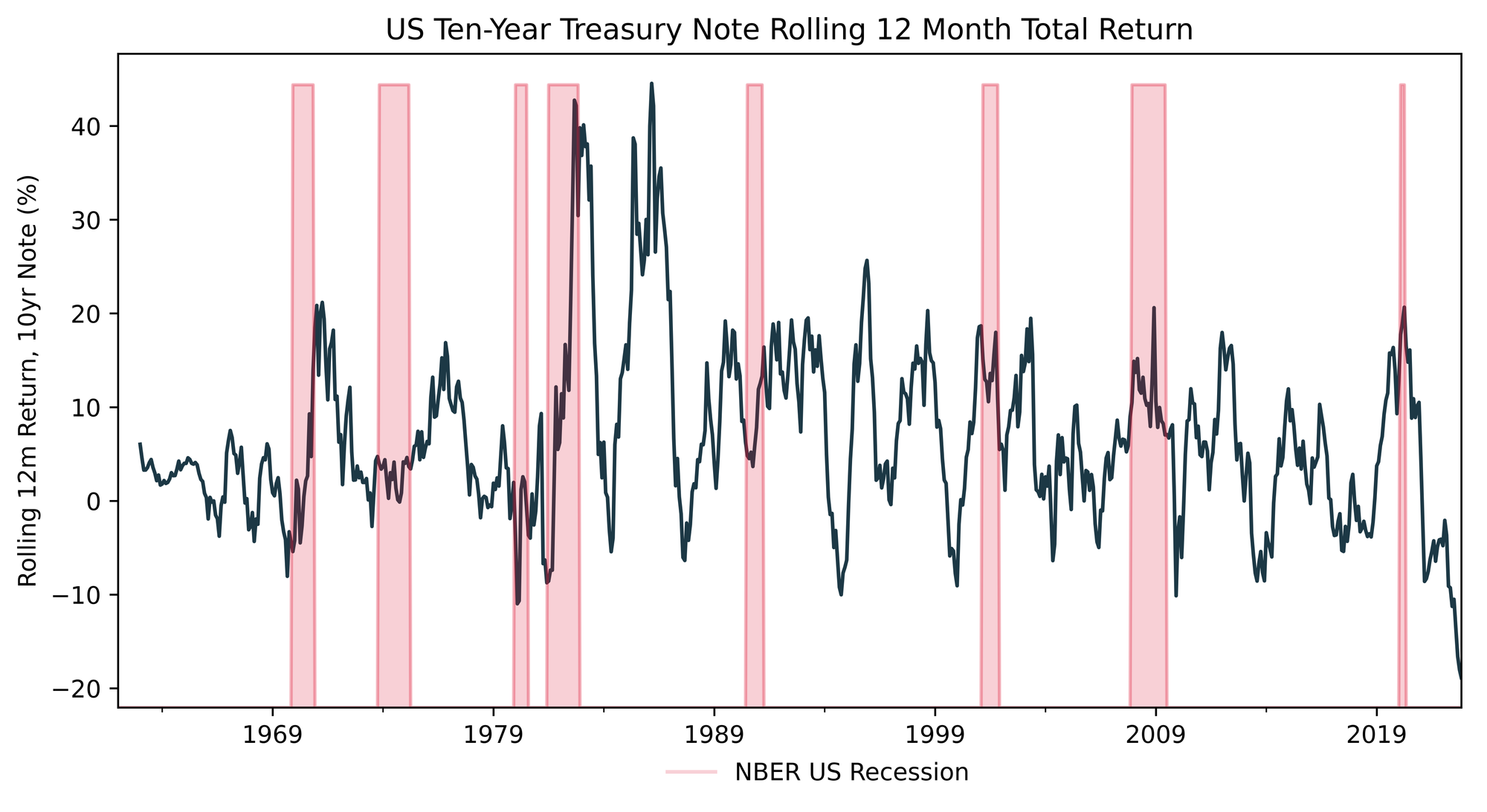
Check out how the relationship changes over time… The emergence of the “Greenspan [and Bernake and Yellen and Powell 1.0] Put” era in the 90’s came with a clear reaction function: economic activity slows or something in the market breaks, leading to aggressive rate cuts and/or a surge in demand for pristine collateral (sweet sweet US Treasuries). This surge in demand causes yields to plummet and pond prices to soar.

We can see these return peaks super clearly over the last three recessions… This phenomenon of negative stock/bond correlation fueled the dominance of the 60/40 portfolio and the rise of more aggressive levered implementations of that theme like risk parity.

Everyone thought they had found financial alchemy: the positive carry hedge (insurance that pays you!). The Achilles heel of that was.. you guessed it.. inflation!

Welp… That’ll do it for our exploration into all things total return. If you missed the first part you can check it out here. Otherwise, stay tuned, plenty more to come from the Lab.

Happy tinkering,

murph

p.s. I am not active on social media. If you’d like to be notified of new tutorials when they drop, consider hopping on my mailing list.